Hive:
- One of biggest ingredients in Information Platform built by Jeffs team at Facebook was Hive
- It is framework for data warehousing on top of Hadoop
- Hive was created to make it possible for analysis with strong SQL skills to run queries on huge volume of data that Facebook stored in HDFS.
Installing Hive:
- Hive runs on your workstation and converts your SQL query into series of MapReduce jobs for execution on Hadoop cluster.
- Hive organized data into tables which provide a means for attaching structure to data stored in HDFS.
- Metadata- such as table schemas- is stored in database called metastore
- It is convenient to run metastore on your local machine.
- Installation of Hive is straightforward. Java 6 is prerequisite and on windows, you need Cygwin, too.
Which versions of Hadoop does Hive work with?
- Any given version of Hive is designed to work with multiple versions of Hadoop.
- Hive works with latest version of Hadoop as well as supporting number of older versions.
- You dont need to do anything special to tell Hive which version of Hadoop you are using, just making sure that hadoop executable is on path or setting HADOOP_HOME environment variable.
- Download release at http://hive.apache.org/releases.html, and unpack the tarball in a
suitable place on your workstation:
% tar xzf hive-x.y.z-dev.tar.gz
It’s handy to put Hive on your path to make it easy to launch:
% export HIVE_INSTALL=/home/tom/hive-x.y.z-dev
% export PATH=$PATH:$HIVE_INSTALL/bin
Now type hive to launch the Hive shell:
% hive
hive>
Hive Shell:
- Shell is primary way to interact with Hive, by issuing commands in HiveQL.
- HiveQL is Hives query language.
- It is heavily influenced by MySQL, so if you are familiar with MySQL you should feel at home using Hive.
-Check whether hive is working by listing its tables:
there should be none.
hive> SHOW TABLES;
OK
Time taken: 10.425 seconds
- Like SQL, HiveQL is generally case insensitive.
- Tab key will autocomplete Hive keywords and functions.
- You can also run Hive shell in non-interactive mode.
- The -f option runs the commands in specified file, script.q, in this example:
% hive -f script.q
For short scripts, you can use the -e option to specify the commands inline, in which
case the final semicolon is not required:
% hive -e 'SELECT * FROM dummy'
Hive history file=/tmp/tom/hive_job_log_tom_201005042112_1906486281.txt
OK
X
Time taken: 4.734 seconds
- Populating single row table:
% echo 'X' > /tmp/dummy.txt
% hive -e "CREATE TABLE dummy (value STRING); \
LOAD DATA LOCAL INPATH '/tmp/dummy.txt' \
OVERWRITE INTO TABLE dummy"
- In both interactive and non-interactive mode, Hive will print information to standard error- such as time taken to run query- during course of operation.
- You can suppress the messages using the -S option at launch time, which shows only output result for queries:
% hive -S -e 'SELECT * FROM dummy'
X
Example:
- Lets use Hive to run query on weather dataset.
- First step is to load data into Hives managed storage.
- We will have Hive use local filesystem for storage.
- Hive organized its data into tables.
- We create table to hold weather data using CREATE TABLE statement:
CREATE TABLE records (year STRING, temperature INT, quality INT)
ROW FORMAT DELIMITED
FIELDS TERMINATED BY '\t';
- First line: declare records table with three columns:
year, temperature and quality.
Type of each column must be specified,too: here year is string, while other two columns are integers.
- The ROW FORMAT clause, however, is particular to HiveQL.
What this declaration is saying is that each row in the data file is tab-delimited text.
Hive expects there to be three fields in each row, corresponding to the table columns,
with fields separated by tabs, and rows by newlines.
- We populate Hive with the data.
LOAD DATA LOCAL INPATH 'input/ncdc/micro-tab/sample.txt'
OVERWRITE INTO TABLE records;
- Running this command tells Hive to put specified local file in its warehouse directory.
- In this ex, we are storing Hive tables on local filesystem(fs.default.name is set to its default value of file:///)/
- Tables are stored as directories under Hives warehouse directory, controlled by hive.metastore.warehouse.dir and defaults to /user/hive/warehouse.
- Thus, files for records table are found in /user/hive/warehouse/records directory on local filesystem:
% ls /user/hive/warehouse/records/
sample.txt
- OVERWRITE keyword in LOAD DATA statement tells Hive to delete any existing files in directory for table.
- If it is ommitted, then new files are simply added to tables directory.
- Now that data is in Hive, we can run query against it:
hive> SELECT year, MAX(temperature)
> FROM records
> WHERE temperature != 9999
> AND (quality = 0 OR quality = 1 OR quality = 4 OR quality = 5 OR quality = 9)
> GROUP BY year;
1949 111
1950 22
- remarkable thing is Hive transforms this query into MapReduce job, which it executes on our behalf, then prints results to console.
Running Hive:
Configuring Hive:
- Hive is configured using XML configuration file like Hadoops.
- The file is called hive-site.xml and is located in Hives conf directory.
- This file is where you can set properties that you want to set everytime you run Hive.
- The same directory contains hive-default.xml which documents properties that Hive exposes and their default values.
- You can override the configuration directory that Hive looks for in hive-site.xml by
passing the --config option to the hive command:
% hive --config /Users/tom/dev/hive-conf
- The hive-site.xml is a natural place to put the cluster connection details: you can specify
the filesystem and jobtracker using the usual Hadoop properties, fs.default.name and
mapred.job.tracker
- Metastore configuration settings (covered in “The Metastore” on page 419) are commonly
found in hive-site.xml
Hive also permits you to set properties on a per-session basis, by passing the
-hiveconf option to the hive command. For example, the following command sets the
cluster (to a pseudo-distributed cluster) for the duration of the session:
% hive -hiveconf fs.default.name=localhost -hiveconf mapred.job.tracker=localhost:8021
If you plan to have more than one Hive user sharing a Hadoop cluster, then
you need to make the directories that Hive uses writable by all
users. The following commands will create the directories and set their
permissions appropriately:
% hadoop fs -mkdir /tmp
% hadoop fs -chmod a+w /tmp
% hadoop fs -mkdir /user/hive/warehouse
% hadoop fs -chmod a+w /user/hive/warehouse
If all users are in the same group, then permissions g+w are sufficient on
the warehouse directory.
You can change settings from within a session, too, using the SET command. This is
useful for changing Hive or MapReduce job settings for a particular query. For example,
the following command ensures buckets are populated according to the table definition
(see “Buckets” on page 430):
hive> SET hive.enforce.bucketing=true;
To see the current value of any property, use SET with just the property name:
hive> SET hive.enforce.bucketing;
hive.enforce.bucketing=true
- Use SET -v to list all the properties in the system,
including Hadoop defaults.
- There is a precedence hierarchy to setting properties. In the following list, lower numbers
take precedence over higher numbers:
1. The Hive SET command
2. The command line -hiveconf option
3. hive-site.xml
4. hive-default.xml
5. hadoop-site.xml (or, equivalently, core-site.xml, hdfs-site.xml, and mapredsite.xml)
6. hadoop-default.xml (or, equivalently, core-default.xml, hdfs-default.xml, and
mapred-default.xml)
Logging:
You can find Hive’s error log on the local file system at /tmp/$USER/hive.log. It can be
very useful when trying to diagnose configuration problems or other types of error.


Semi Joins:
- Hive does not support IN subqueries, but you can use a LEFT SEMIJOIN to do the same thing.
Consider this IN subquery, which finds all the items in the things table that are in the
sales table:
SELECT *
FROM things
WHERE things.id IN (SELECT id from sales);
We can rewrite it as follows:
hive> SELECT *
> FROM things LEFT SEMI JOIN sales ON (sales.id = things.id);
2 Tie
3 Hat
4 Coat
There is a restriction that we must observe for LEFT SEMI JOIN queries: the right table
(sales) may only appear in the ON clause. It cannot be referenced in a SELECT expression,
for example.
Map Joins:
- If one table is small enough to fit in memory, then Hive can load the smaller table into
memory to perform the join in each of the mappers. The syntax for specifying a map
join is a hint embedded in an SQL C-style comment:
SELECT /*+ MAPJOIN(things) */ sales.*, things.*
FROM sales JOIN things ON (sales.id = things.id);
The job to execute this query has no reducers, so this query would not work for a
RIGHT or FULL OUTER JOIN, since absence of matching can only be detected in an aggregating
(reduce) step across all the inputs.
Map joins can take advantage of bucketed tables (“Buckets” on page 430), since a
mapper working on a bucket of the left table only needs to load the corresponding
buckets of the right table to perform the join. The syntax for the join is the same as for
the in-memory case above; however, you also need to enable the optimization with:
SET hive.optimize.bucketmapjoin=true;
Subqueries:
- select statement embedded in another SQL statement.
- Hive has limited support for subqueries, only permitting subquery in the FROM clause of SELECT statement.
The following query finds the mean maximum temperature for every year and weather
station:
SELECT station, year, AVG(max_temperature)
FROM (
SELECT station, year, MAX(temperature) AS max_temperature
FROM records2
WHERE temperature != 9999
AND (quality = 0 OR quality = 1 OR quality = 4 OR quality = 5 OR quality = 9)
GROUP BY station, year
) mt
GROUP BY station, year;
The subquery is used to find the maximum temperature for each station/date combination,
then the outer query uses the AVG aggregate function to find the average of the maximum
temperature readings for each station/date combination.
- One of biggest ingredients in Information Platform built by Jeffs team at Facebook was Hive
- It is framework for data warehousing on top of Hadoop
- Hive was created to make it possible for analysis with strong SQL skills to run queries on huge volume of data that Facebook stored in HDFS.
Installing Hive:
- Hive runs on your workstation and converts your SQL query into series of MapReduce jobs for execution on Hadoop cluster.
- Hive organized data into tables which provide a means for attaching structure to data stored in HDFS.
- Metadata- such as table schemas- is stored in database called metastore
- It is convenient to run metastore on your local machine.
- Installation of Hive is straightforward. Java 6 is prerequisite and on windows, you need Cygwin, too.
Which versions of Hadoop does Hive work with?
- Any given version of Hive is designed to work with multiple versions of Hadoop.
- Hive works with latest version of Hadoop as well as supporting number of older versions.
- You dont need to do anything special to tell Hive which version of Hadoop you are using, just making sure that hadoop executable is on path or setting HADOOP_HOME environment variable.
- Download release at http://hive.apache.org/releases.html, and unpack the tarball in a
suitable place on your workstation:
% tar xzf hive-x.y.z-dev.tar.gz
It’s handy to put Hive on your path to make it easy to launch:
% export HIVE_INSTALL=/home/tom/hive-x.y.z-dev
% export PATH=$PATH:$HIVE_INSTALL/bin
Now type hive to launch the Hive shell:
% hive
hive>
Hive Shell:
- Shell is primary way to interact with Hive, by issuing commands in HiveQL.
- HiveQL is Hives query language.
- It is heavily influenced by MySQL, so if you are familiar with MySQL you should feel at home using Hive.
-Check whether hive is working by listing its tables:
there should be none.
hive> SHOW TABLES;
OK
Time taken: 10.425 seconds
- Like SQL, HiveQL is generally case insensitive.
- Tab key will autocomplete Hive keywords and functions.
- You can also run Hive shell in non-interactive mode.
- The -f option runs the commands in specified file, script.q, in this example:
% hive -f script.q
For short scripts, you can use the -e option to specify the commands inline, in which
case the final semicolon is not required:
% hive -e 'SELECT * FROM dummy'
Hive history file=/tmp/tom/hive_job_log_tom_201005042112_1906486281.txt
OK
X
Time taken: 4.734 seconds
- Populating single row table:
% echo 'X' > /tmp/dummy.txt
% hive -e "CREATE TABLE dummy (value STRING); \
LOAD DATA LOCAL INPATH '/tmp/dummy.txt' \
OVERWRITE INTO TABLE dummy"
- In both interactive and non-interactive mode, Hive will print information to standard error- such as time taken to run query- during course of operation.
- You can suppress the messages using the -S option at launch time, which shows only output result for queries:
% hive -S -e 'SELECT * FROM dummy'
X
Example:
- Lets use Hive to run query on weather dataset.
- First step is to load data into Hives managed storage.
- We will have Hive use local filesystem for storage.
- Hive organized its data into tables.
- We create table to hold weather data using CREATE TABLE statement:
CREATE TABLE records (year STRING, temperature INT, quality INT)
ROW FORMAT DELIMITED
FIELDS TERMINATED BY '\t';
- First line: declare records table with three columns:
year, temperature and quality.
Type of each column must be specified,too: here year is string, while other two columns are integers.
- The ROW FORMAT clause, however, is particular to HiveQL.
What this declaration is saying is that each row in the data file is tab-delimited text.
Hive expects there to be three fields in each row, corresponding to the table columns,
with fields separated by tabs, and rows by newlines.
- We populate Hive with the data.
LOAD DATA LOCAL INPATH 'input/ncdc/micro-tab/sample.txt'
OVERWRITE INTO TABLE records;
- Running this command tells Hive to put specified local file in its warehouse directory.
- In this ex, we are storing Hive tables on local filesystem(fs.default.name is set to its default value of file:///)/
- Tables are stored as directories under Hives warehouse directory, controlled by hive.metastore.warehouse.dir and defaults to /user/hive/warehouse.
- Thus, files for records table are found in /user/hive/warehouse/records directory on local filesystem:
% ls /user/hive/warehouse/records/
sample.txt
- OVERWRITE keyword in LOAD DATA statement tells Hive to delete any existing files in directory for table.
- If it is ommitted, then new files are simply added to tables directory.
- Now that data is in Hive, we can run query against it:
hive> SELECT year, MAX(temperature)
> FROM records
> WHERE temperature != 9999
> AND (quality = 0 OR quality = 1 OR quality = 4 OR quality = 5 OR quality = 9)
> GROUP BY year;
1949 111
1950 22
- remarkable thing is Hive transforms this query into MapReduce job, which it executes on our behalf, then prints results to console.
Running Hive:
Configuring Hive:
- Hive is configured using XML configuration file like Hadoops.
- The file is called hive-site.xml and is located in Hives conf directory.
- This file is where you can set properties that you want to set everytime you run Hive.
- The same directory contains hive-default.xml which documents properties that Hive exposes and their default values.
- You can override the configuration directory that Hive looks for in hive-site.xml by
passing the --config option to the hive command:
% hive --config /Users/tom/dev/hive-conf
- The hive-site.xml is a natural place to put the cluster connection details: you can specify
the filesystem and jobtracker using the usual Hadoop properties, fs.default.name and
mapred.job.tracker
- Metastore configuration settings (covered in “The Metastore” on page 419) are commonly
found in hive-site.xml
Hive also permits you to set properties on a per-session basis, by passing the
-hiveconf option to the hive command. For example, the following command sets the
cluster (to a pseudo-distributed cluster) for the duration of the session:
% hive -hiveconf fs.default.name=localhost -hiveconf mapred.job.tracker=localhost:8021
If you plan to have more than one Hive user sharing a Hadoop cluster, then
you need to make the directories that Hive uses writable by all
users. The following commands will create the directories and set their
permissions appropriately:
% hadoop fs -mkdir /tmp
% hadoop fs -chmod a+w /tmp
% hadoop fs -mkdir /user/hive/warehouse
% hadoop fs -chmod a+w /user/hive/warehouse
If all users are in the same group, then permissions g+w are sufficient on
the warehouse directory.
You can change settings from within a session, too, using the SET command. This is
useful for changing Hive or MapReduce job settings for a particular query. For example,
the following command ensures buckets are populated according to the table definition
(see “Buckets” on page 430):
hive> SET hive.enforce.bucketing=true;
To see the current value of any property, use SET with just the property name:
hive> SET hive.enforce.bucketing;
hive.enforce.bucketing=true
- Use SET -v to list all the properties in the system,
including Hadoop defaults.
- There is a precedence hierarchy to setting properties. In the following list, lower numbers
take precedence over higher numbers:
1. The Hive SET command
2. The command line -hiveconf option
3. hive-site.xml
4. hive-default.xml
5. hadoop-site.xml (or, equivalently, core-site.xml, hdfs-site.xml, and mapredsite.xml)
6. hadoop-default.xml (or, equivalently, core-default.xml, hdfs-default.xml, and
mapred-default.xml)
Logging:
You can find Hive’s error log on the local file system at /tmp/$USER/hive.log. It can be
very useful when trying to diagnose configuration problems or other types of error.
- Logging configuration is in conf/hive-log4j.properties and you can edit this file to change log levels and other logging related settings.
- Often though, it’s more convenient
to set logging configuration for the session. For example, the following handy invocation
will send debug messages to the console:
% hive -hiveconf hive.root.logger=DEBUG,console
Hive Services:
- Hive shell is only one of several services you run using hive command.
- You can specify service to run using --service option.
- Type hive --service help to get list of available service names
cli
The command line interface to Hive (the shell). This is the default service.
hiveserver
Runs Hive as a server exposing a Thrift service, enabling access from a range of
clients written in different languages. Applications using the Thrift, JDBC, and
ODBC connectors need to run a Hive server to communicate with Hive. Set the
HIVE_PORT environment variable to specify the port the server will listen on (defaults
to 10,000).
hwi
The Hive Web Interface. See “The Hive Web Interface (HWI)” on page 418.
jar
The Hive equivalent to hadoop jar, a convenient way to run Java applications that
includes both Hadoop and Hive classes on the classpath.
metastore
By default, the metastore is run in the same process as the Hive service. Using this service, it is possible to run the metastore as a standalone (remote) process. Set the METASTORE_PORT environment variable to specify the port the server will listen on.
As an alternative to the shell, you might want to try Hive’s simple web interface. Start
it using the following commands:
% export ANT_LIB=/path/to/ant/lib
% hive --service hwi
(You only need to set the ANT_LIB environment variable if Ant’s library is not found
in /opt/ant/lib on your system.) Then navigate to http://localhost:9999/hwi in your
browser. From there, you can browse Hive database schemas and create sessions for
issuing commands and queries.
Hive Clients:
- If you run Hive as server(hive --service hiveserver), then there are number of different mechanism for connecting it from applications.
Thrift client:
- The Hive Thrift Client makes it easy to run Hive commands from a wide range of
programming languages. Thrift bindings for Hive are available for C++, Java, PHP,
Python, and Ruby. They can be found in the src/service/src subdirectory in the Hive
distribution.
JDBC Driver:
Hive provides a Type 4 (pure Java) JDBC driver, defined in the class
org.apache.hadoop.hive.jdbc.HiveDriver. When configured with a JDBC URI of
the form jdbc:hive://host:port/dbname, a Java application will connect to a Hive
server running in a separate process at the given host and port. (The driver makes
calls to an interface implemented by the Hive Thrift Client using the Java Thrift
bindings.)
You may alternatively choose to connect to Hive via JDBC in embedded mode using
the URI jdbc:hive://. In this mode, Hive runs in the same JVM as the application
invoking it, so there is no need to launch it as a standalone server since it does not
use the Thrift service or the Hive Thrift Client.
ODBC Driver:
The Hive ODBC Driver allows applications that support the ODBC protocol to
connect to Hive. (Like the JDBC driver, the ODBC driver uses Thrift to communicate
with the Hive server.)
The ODBC driver is still in development, so you should refer
to the latest instructions on the Hive wiki for how to build and run it.
Metastore:
- Central repository of Hive metadata.
- The metastore is divided into
two pieces: a service and the backing store for the data. By default, the metastore service
runs in the same JVM as the Hive service and contains an embedded Derby database
instance backed by the local disk. This is called the embedded metastore configuration
(see Figure 12-2).
Using an embedded metastore is a simple way to get started with Hive; however, only
one embedded Derby database can access the database files on disk at any one time,
which means you can only have one Hive session open at a time that shares the same
metastore. Trying to start a second session gives the error:
Failed to start database 'metastore_db'
when it attempts to open a connection to the metastore.
The solution to supporting multiple sessions (and therefore multiple users) is to use a
standalone database. This configuration is referred to as a local metastore, since the
metastore service still runs in the same process as the Hive service, but connects to a
database running in a separate process, either on the same machine or on a remote machine.
MySQL is a popular choice for the standalone metastore. In this case,
javax.jdo.option.ConnectionURL is set to jdbc:mysql://host/dbname?createDatabaseIf
NotExist=true, and javax.jdo.option.ConnectionDriverName is set to
com.mysql.jdbc.Driver.
Going a step further, there’s another metastore configuration called a remote metastore,
where one or more metastore servers run in separate processes to the Hive service.
This brings better manageability and security, since the database tier can be completely
firewalled off, and the clients no longer need the database credentials.
Schema on Read Versus Schema on Write:
- In traditional database, design is sometimes called schema on write, since data is checked against schema when it is written into database.
- Hive does not verify data when it is loaded, but rather when query is issued. This is called schema on read.
- Schema on read makes for very fast initial load, since data does not have to be read, parsed, and serialized to disk in databases internal format.
- Load operation is just file copy or move.
- Schema on write makes query time performance faster, since DB can index columns and perform compression on data. It takes longer to load data in database.
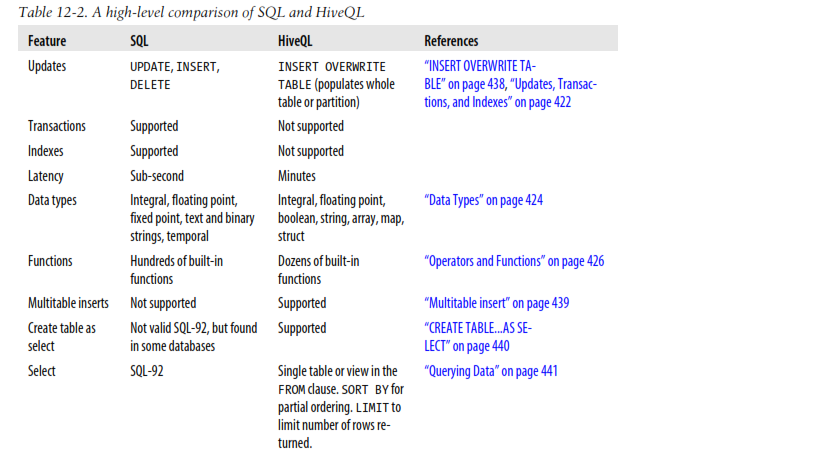
Updates, Transactions and Indexes:
- These features have not been considered part of Hives feature set.
- This is as Hive was built to operate over HDFS data using MapReduce where full table scans are norm and table update is achieved by transforming data into new table.
HiveQL:
- In fact, to first order approxmation, HiveQL most closely resembles MySQLs SQL dialect.
- Some of Hives extensions to SQL-92 were inspired by MapReduce, such as multitable inserts and the TRANSFORM, MAP and REDUCE clauses.
Data Types:
- Hive supports both primitive and complex data type.
- Primitive: boolean, numeric, string and timestamp types.
- Complex: arrays, maps and structs.
Complex Types :
Hive has three complex types:
- ARRAY
- MAP
- STRUCT
- ARRAY and MAP are like namesakes in Java
- STRUCT is record type that encapsulates set of named fields.
- CREATE TABLE complex (
col1 ARRAY<INT>,
col2 MAP<STRING, INT>,
col3 STRUCT<a:STRING, b:INT, c:DOUBLE>
);
If we load the table with one row of data for ARRAY, MAP, and STRUCT shown in the “Literal
examples” column in Table 12-3 (we’ll see the file format needed to do this in “Storage
Formats” on page 433), then the following query demonstrates the field accessor
operators for each type:
hive> SELECT col1[0], col2['b'], col3.c FROM complex;
1 2 1.0
Operators and Functions:
- Hive comes with a large number of built-in functions—too many to list here—divided
into categories including mathematical and statistical functions, string functions, date
functions (for operating on string representations of dates), conditional functions, ag-
gregate functions, and functions for working with XML (using the xpath function) and
JSON.
You can retrieve a list of functions from the Hive shell by typing SHOW FUNCTIONS.
To
get brief usage instructions for a particular function, use the DESCRIBE command:
hive> DESCRIBE FUNCTION length;
length(str) - Returns the length of str
In the case when there is no built-in function that does what you want, you can write
your own.
Tables:
- Hive table is logically made up of data being stored and associated metadata describing the layout of the data in table.
- Data typically resides in HDFS, although it may reside in any Hadoop filesystem, including local filesystem or S3.
- Hive stores metadata in relational database not in HDFS.
- If no database is specified, tables belong to the default database.
Managed Tables and External Tables:
- When you create table in Hive, by default Hive will manage the data, which means that Hive moves the data into its warehouse directory.
- Alternately, we can create external table.
- Difference between two types of table is seen in the LOAD and DROP semantics.
- When you load data into managed table, it is moved into Hives warehouse directory.
CREATE TABLE managed_table (dummy STRING);
LOAD DATA INPATH '/user/tom/data.txt' INTO table managed_table;
will move the file hdfs://user/tom/data.txt into Hives warehouse directory for managed_table table.
- If table is later dropped, using:
DROP TABLE managed_table;
then table, including its metadata and its data is deleted.
- An external table behaves differently. You control the creation and deletion of the data.
Location of the external data is specified at table creation time:
CREATE EXTERNAL TABLE external_table (dummy STRING)
LOCATION '/user/tom/external_table';
LOAD DATA INPATH '/user/tom/data.txt' INTO TABLE external_table;
- With the external keyword, Hive knows that it is not managing the data, so it does not move it to its warehouse directory.
- It does not even check if external location exists at the time it is defined.
- This is useful when you create the data lazily after creating the table.
- When you drop an external table, Hive will leave the data untouched and only delete the metadata.
- If you are doing all your processing with Hive, then use managed table.
- If you wish to use Hive and other tools on the same dataset, then use external tables.
- Common pattern is to use external table to access an initial dataset stored in HDFS, then use Hive transform to move data into managed Hive table.
- External table can be used to export data from Hive to other applications to use.
- Another reason to use external tables is when you wish to associate multiple schemas with same dataset.
Partition and Buckets:
- Hive organizes tables into partitions, way of dividing table into coarse grained parts based on value of partition column, such as date.
- Using partitions can make it fasted to do queries on slices of the data.
- Table or partitions may be subdivide into bucket, to give extra structure to the data that may be used for more efficient queries.
- For ex, bucketing by user ID means we can quickly evaluate user based query by running it on randomized sample of total set of users.
Partitions:
- Imagine a log files where each record includes a timestamp.
- If we partitioned by date, then records for the same date would be stored in same partition.
- Advantage of this schema is that queries that are restricted to particular date or set of dates can be answered much more efficiently since they only need to scan files in partitions that query pertains to.
- Using partition it is still possible to query entire dataset across many partitions.
- Table can be partitioned in multiple dimensions.
- In addition to partitioning logs by date, we might also subpartition each date partition by country to permit efficient queries by location.
- Partitions are defined at table creation time using the PARTITIONED BY clause, which takes list of column definitions.
- For hypothetical log files example, we might define a table with records comprising timestamp and log line itself:
CREATE TABLE logs (ts BIGINT, line STRING)
PARTITIONED BY (dt STRING, country STRING);
- When we load data into partitioned table, partition values are specified explicitly:
LOAD DATA LOCAL INPATH 'input/hive/partitions/file1'
INTO TABLE logs
PARTITION (dt='2001-01-01', country='GB');
- Partitions are simple nested subdirectories of table directory.
- After loading few more lines into logs table, directory structure might look like this:
/user/hive/warehouse/logs/dt=2010-01-01/country=GB/file1
/file2
/country=US/file3
/dt=2010-01-02/country=GB/file4
/country=US/file5
/file6
- logs table has two date paritions: 2010-01-01
and 2010-01-02 corresponding to subdirectories called dt=2010-01-01 and dt=2010-01-02 and two country subpartitions, GB and US, corresponding to nested subdirectories called country = GB and country = US. Data files reside in the leaf directories.
- We can ask Hive for partitions in table using SHOW PARTITIONS:
hive> SHOW PARTITIONS logs;
dt=2001-01-01/country=GB
dt=2001-01-01/country=US
dt=2001-01-02/country=GB
dt=2001-01-02/country=US
- Column definitions in PARTITIONED BY clause are full fledged table columns, called partition columns, however, data files do not contain values for these columns since they are derived from directory names.
- You can use partition columns in SELECT statements in usual way.
- Hive performs input pruning to scan only the relevant partitions.
For ex:
SELECT ts, dt, line
FROM logs
WHERE country='GB';
will only scan file1, file2 and file4.
Buckets:
- Two reasons why you want to organize tables into buckets.
- To enable more efficient queries. Join of two tables that are bucketed on same columns- which include the join columns- can be efficiently implemented as map-side join.
- To make sampling more efficient.
- Lets see how to tell Hive that table should be bucketed.
- We use the CLUSTERED BY clause to specify columns to bucket on and number of buckets:
CREATE TABLE bucketed_users (id INT, name STRING)
CLUSTERED BY (id) INTO 4 BUCKETS;
- Here are we using the user ID to determine the bucket, so any particular bucket will effectively have random set of users to it.
- The data in the bucket may be sorted by one or more columns.
- The syntax for declaring that table has sorted buckets is:
CREATE TABLE bucketed_users (id INT, name STRING)
CLUSTERED BY (id) SORTED BY (id ASC) INTO 4 BUCKETS;
Take an unbucketed users table:
hive> SELECT * FROM users;
0 Nat
2 Joe
3 Kay
4 Ann
To populate the bucketed table, we need to set the hive.enforce.bucketing property to true, so that Hive knows to create number of buckets declared in table definition. Then it is matter of just using the INSERT command:
INSERT OVERWRITE TABLE bucketed_users
SELECT * FROM users;
- Physically each bucket is just a file in table directory.
- In fact buckets correspond to MapReduce output file partitions: a job will produce as many buckets(output files) as reduce tasks.
- We can see this by looking at the layout of the bucketed_users table we just created.
Running this command:
hive> dfs -ls /user/hive/warehouse/bucketed_users;
shows that four files were created, with following names
attempt_201005221636_0016_r_000000_0
attempt_201005221636_0016_r_000001_0
attempt_201005221636_0016_r_000002_0
attempt_201005221636_0016_r_000003_0
- First bucket contains the users with IDs 0 and 4, since for an INT the hash is the integer itself, and value is reduced modulo the number of buckets - 4 in this case:
hive> dfs -cat /user/hive/warehouse/bucketed_users/*0_0;
0Nat
4Ann
We can see the same thing by sampling the table using the TABLESAMPLE clause, which
restricts the query to a fraction of the buckets in the table rather than the whole table:
hive> SELECT * FROM bucketed_users
> TABLESAMPLE(BUCKET 1 OUT OF 4 ON id);
0 Nat
4 Ann
For ex, this query returns half of the buckets:
hive> SELECT * FROM bucketed_users
> TABLESAMPLE(BUCKET 1 OUT OF 2 ON id);
0 Nat
4 Ann
2 Joe
Sampling a bucketed table is very efficient, since the whole query only has to read the buckets that match the TABLESAMPLE clause.
- Contrast this with sampling a non bucketed table using the rand() function, where the whole input dataset is scanned, even if a very small sample is needed:
hive> SELECT * FROM users
> TABLESAMPLE(BUCKET 1 OUT OF 4 ON rand());
2 Joe
Storage formats:
- There are two dimensions that govern table storage in Hive: the row format and file format.
- Row format dictates how rows and fields in particular row are stored.
- In Hive, row format is defined by SerDe.
- File format dictates the container format for fields in a row.
- Simplest format is plain text file, but there are row oriented and column oriented binary formats available too.
Default storage format: Delimited text
The statement:
CREATE TABLE ...;
is identical to the more explicit:
CREATE TABLE ...
ROW FORMAT DELIMITED
FIELDS TERMINATED BY '\001'
COLLECTION ITEMS TERMINATED BY '\002'
MAP KEYS TERMINATED BY '\003'
LINES TERMINATED BY '\n'
STORED AS TEXTFILE;
Binary Storage Format: Sequence files and RCFiles:
- Hadoops sequence file format is general purpose binary format for sequences of records(key-value pairs).
- You can use sequence files in Hive by using the declaration STORED AS SEQUENCEFILES in the CREATE TABLE statement.
- One of the main benefits of using sequence files is their support for splittable compression.
- If you have collection of sequence files that were created outside Hive, then Hive will read them with no extra configuration.
- If you want tables populated from Hive to use compressed sequence files for their storage, you need to set few properties to enable compression:
hive> SET hive.exec.compress.output=true;
hive> SET mapred.output.compress=true;
hive> SET mapred.output.compression.codec=org.apache.hadoop.io.compress.GzipCodec;
hive> INSERT OVERWRITE TABLE ...;
Hive provides another binary storage format called RCFile, short for Record columnar File.
- RCFiles are similar to sequence files, except that they store data in column oriented fashion.
- RCFile breaks up the table into row splits, then within each split stores the values for each row in first column, followed by the values for each row in second column
- With column oriented storage , only the column 2 parts of the file need to be read into memory.
Use the following CREATE TABLE clauses to enable column-oriented storage in Hive:
CREATE TABLE ...
ROW FORMAT SERDE 'org.apache.hadoop.hive.serde2.columnar.ColumnarSerDe'
STORED AS RCFILE;
Example: RegexSerDe
- We’ll use a contrib SerDe that uses a regular expression for reading the fixed-width station metadata from a text file:
CREATE TABLE stations (usaf STRING, wban STRING, name STRING)
ROW FORMAT SERDE 'org.apache.hadoop.hive.contrib.serde2.RegexSerDe'
WITH SERDEPROPERTIES (
"input.regex" = "(\\d{6}) (\\d{5}) (.{29}) .*"
);
- In this example, we specify SerDe with the SERDE keyword and fully qualified classname of the Java class that implements the SerDe, org.apache.hadoop.hive.contrib.serde2.RegexSerDe.
- SerDes can be configured with extra properties using the WITH SERDEPROPERTIES clause.
- Here we set the input.regex property, which is specific to RegexSerDe.
- input.regex is regular expression pattern to be used during deserialization to turn line of text forming row into a set of columns.
To populate the table, we use the LOAD DATA statement as before:
LOAD DATA LOCAL INPATH "input/ncdc/metadata/stations-fixed-width.txt"
INTO TABLE stations;
When we retrieve data from the table, the SerDe is invoked for deserialization, as we
can see from this simple query, which correctly parses the fields for each row:
hive> SELECT * FROM stations LIMIT 4;
010000 99999 BOGUS NORWAY
010003 99999 BOGUS NORWAY
010010 99999 JAN MAYEN
010013 99999 ROST
Importing Data:
- You can also populate table with data from another Hive table using an INSERT statement, or at creation time using the CTAS construct,which is an abbreviation used to refer to CREATE TABLE...AS SELECT
- If you want to import data from relational database directly into Hive, have a look as Sqoop.
INSERT OVERWRITE TABLE
- Here is an example of an INSERT statement:
INSERT OVERWRITE TABLE target
SELECT col1, col2
FROM source;
- For partitioned tables, you can specify the partition to insert into by supplying PARTITION clause:
INSERT OVERWRITE TABLE target
PARTITION (dt='2010-01-01')
SELECT col1, col2
FROM source;
- OVERWRITE keyword is actually mandatory in both cases, and means that the contents of the target table or the 2010-01-01 partition are replaced by results of the SELECT statement.
- You can specify the partition dynamically, by determining the partition value from the SELECT statement:
INSERT OVERWRITE TABLE target
PARTITION (dt)
SELECT col1, col2, dt
FROM source;
- This is known as dynamic partition insert.
- This feature is off by default, so you need to enable it by setting hive.exec.dynamic.partition to true first.
Multitable insert:
- In HiveQL, you can turn the INSERT statement around and start with FROM clause for same effect:
FROM source
INSERT OVERWRITE TABLE target
SELECT col1, col2;
- Reason for this syntax is clear when you see that its possible to have multiple INSERT clauses in same query.
- This so called multitable insert is more efficient than multiple INSERT statements, since source table need only be scanned once to produce the multiple disjoint outputs.
Here’s an example that computes various statistics over the weather dataset:
FROM records2
INSERT OVERWRITE TABLE stations_by_year
SELECT year, COUNT(DISTINCT station)
GROUP BY year
INSERT OVERWRITE TABLE records_by_year
SELECT year, COUNT(1)
GROUP BY year
INSERT OVERWRITE TABLE good_records_by_year
SELECT year, COUNT(1)
WHERE temperature != 9999
AND (quality = 0 OR quality = 1 OR quality = 4 OR quality = 5 OR quality = 9)
GROUP BY year;
- There is single source table(records 2), but three tables to hold the results from three different queries over the source.
CREATE TABLE....AS SELECT
- Its often very convenient to store output of Hive query in new table, as it is too large to be dumped to console as there are further processing steps to carry out on the result.
- The new table’s column definitions are derived from the columns retrieved by the
SELECT clause. In the following query, the target table has two columns named col1
and col2 whose types are the same as the ones in the source table:
CREATE TABLE target
AS
SELECT col1, col2
FROM source;
A CTAS operation is atomic, so if the SELECT query fails for some reason, then the table
is not created.
Altering Tables:
- You can rename a table using the ALTER TABLE statement:
ALTER TABLE source RENAME TO target;
Hive allows you to change the definition for columns, add new columns, or even replace
all existing columns in a table with a new set.
For example, consider adding a new column:
ALTER TABLE target ADD COLUMNS (col3 STRING);
- Since Hive does not permit updating existing records, you will need to arrange for underlying files to be updated by another mechanism.
- For this reason, it is more common to create a new table that defines new columns and populates them using the SELECT statement.
- To learn more about how to alter a table’s structure, including adding and dropping
partitions, changing and replacing columns, and changing table and SerDe properties,
see the Hive wiki at https://cwiki.apache.org/confluence/display/Hive/LanguageManual
+DDL.
Dropping tables:
- DROP TABLE statement deletes the data and metadata for table.
- In case of external table, only metadata is deleted- data is left untouched,
- If you want to delete all the data in a table, but keep the table definition (like DELETE or
TRUNCATE in MySQL), then you can simply delete the data files. For example:
hive> dfs -rmr /user/hive/warehouse/my_table;
Hive treats a lack of files (or indeed no directory for the table) as an empty table.
Another possibility, which achieves a similar effect, is to create a new, empty table that
has the same schema as the first, using the LIKE keyword:
CREATE TABLE new_table LIKE existing_table;
Querying Data:
Sorting and Aggregating:
- Sorting data in Hive can be achieved by use of standard ORDER BY clause, but there is a catch.
- ORDER BY produces result that is totally sorted, as expected, but to do so it sets number of reducers to one, making it very inefficient for large datasets.
- When globally sorted result is not required- then you can use Hive nonstandard extension, SORT BY instead. SORT BY produces a sorted file per reducer.
- In some cases, you want to control which reducer particular row goes to, so you can perform some subsequent aggregation.
- This is what Hives DISTRIBUTE BY clause does.
- Here’s an example to sort the weather dataset by year and temperature, in
such a way to ensure that all the rows for a given year end up in the same reducer
partition:
hive> FROM records2
> SELECT year, temperature
> DISTRIBUTE BY year
> SORT BY year ASC, temperature DESC;
1949 111
1949 78
1950 22
1950 0
1950 -11
If the columns for SORT BY and DISTRIBUTE BY are the same, you can use CLUSTER BY as
a shorthand for specifying both.
MapReduce scripts:
Suppose we want to use a script to filter out rows that don’t meet some condition, such as the script in Example, which removes poor quality readings.
Example: Python script to filter out poor quality weather records
#!/usr/bin/env python
import re
import sys
for line in sys.stdin:
(year, temp, q) = line.strip().split()
if (temp != "9999" and re.match("[01459]", q)):
print "%s\t%s" % (year, temp)
We can use the script as follows:
hive> ADD FILE /path/to/is_good_quality.py;
hive> FROM records2
> SELECT TRANSFORM(year, temperature, quality)
> USING 'is_good_quality.py'
> AS year, temperature;
1949 111
1949 78
1950 0
1950 22
1950 -11
- Before running the query, we need to register script with Hive.
- This is so Hive knows to ship the file to Hadoop cluster.
This example has no reducers. If we use a nested form for the query, we can specify a
map and a reduce function. This time we use the MAP and REDUCE keywords, but SELECT
TRANSFORM in both cases would have the same result. The source for the max_temperature_reduce.py
script is shown in Example :
FROM (
FROM records2
MAP year, temperature, quality
USING 'is_good_quality.py'
AS year, temperature) map_output
REDUCE year, temperature
USING 'max_temperature_reduce.py'
AS year, temperature;
Joins:
- Hive makes commonly used operations very simple.
Inner Joins:
- Each match in the input table results in a row in the output.
- Consider two small demonstration tables: sales which lists names of people and the ID of the item they bought, and things, which lists the item ID and its name:
hive> SELECT * FROM sales;
Joe 2
Hank 4
Ali 0
Eve 3
Hank 2
hive> SELECT * FROM things;
2 Tie
4 Coat
3 Hat
1 Scarf
- We can perform inner join on two tables as follows:
hive> SELECT sales.*, things.*
> FROM sales JOIN things ON (sales.id = things.id);
Joe 2 2 Tie
Hank 2 2 Tie
Eve 3 3 Hat
Hank 4 4 Coat
- Hive only supports equijoins, which means that only equality can be used in join predicate, which here matches on the id column in both tables.
You can see how many MapReduce jobs Hive will use for any particular
query by prefixing it with the EXPLAIN
keyword:
EXPLAIN
SELECT sales.*, things.*
FROM sales JOIN things ON (sales.id = things.id);
The EXPLAIN output includes many details about the execution plan for the query, including
the abstract syntax tree, the dependency graph for the stages that Hive will
execute, and information about each stage. Stages may be MapReduce jobs or operations
such as file moves.
For even more detail, prefix the query with EXPLAIN EXTENDED.
Outer joins:
- Outer joins allow you to find nonmatches in the tables being joined. In the current
example, when we performed an inner join, the row for Ali did not appear in the output,
since the ID of the item she purchased was not present in the things table. If we change
the join type to LEFT OUTER JOIN, then the query will return a row for every row in the
left table (sales), even if there is no corresponding row in the table it is being joined to
(things):
hive> SELECT sales.*, things.*
> FROM sales LEFT OUTER JOIN things ON (sales.id = things.id);
Ali 0 NULL NULL
Joe 2 2 Tie
Hank 2 2 Tie
Eve 3 3 Hat
Hank 4 4 Coat
Hive supports right outer joins, which reverses the roles of the tables relative to the left
join. In this case, all items from the things table are included, even those that weren’t
purchased by anyone (a scarf):
hive> SELECT sales.*, things.*
> FROM sales RIGHT OUTER JOIN things ON (sales.id = things.id);
NULL NULL 1 Scarf
Joe 2 2 Tie
Hank 2 2 Tie
Eve 3 3 Hat
Hank 4 4 Coat
Finally, there is a full outer join, where the output has a row for each row from both
tables in the join:
hive> SELECT sales.*, things.*
> FROM sales FULL OUTER JOIN things ON (sales.id = things.id);
Ali 0 NULL NULL
NULL NULL 1 Scarf
Joe 2 2 Tie
Hank 2 2 Tie
Eve 3 3 Hat
Hank 4 4 Coat
- Hive does not support IN subqueries, but you can use a LEFT SEMIJOIN to do the same thing.
Consider this IN subquery, which finds all the items in the things table that are in the
sales table:
SELECT *
FROM things
WHERE things.id IN (SELECT id from sales);
We can rewrite it as follows:
hive> SELECT *
> FROM things LEFT SEMI JOIN sales ON (sales.id = things.id);
2 Tie
3 Hat
4 Coat
There is a restriction that we must observe for LEFT SEMI JOIN queries: the right table
(sales) may only appear in the ON clause. It cannot be referenced in a SELECT expression,
for example.
Map Joins:
- If one table is small enough to fit in memory, then Hive can load the smaller table into
memory to perform the join in each of the mappers. The syntax for specifying a map
join is a hint embedded in an SQL C-style comment:
SELECT /*+ MAPJOIN(things) */ sales.*, things.*
FROM sales JOIN things ON (sales.id = things.id);
The job to execute this query has no reducers, so this query would not work for a
RIGHT or FULL OUTER JOIN, since absence of matching can only be detected in an aggregating
(reduce) step across all the inputs.
Map joins can take advantage of bucketed tables (“Buckets” on page 430), since a
mapper working on a bucket of the left table only needs to load the corresponding
buckets of the right table to perform the join. The syntax for the join is the same as for
the in-memory case above; however, you also need to enable the optimization with:
SET hive.optimize.bucketmapjoin=true;
Subqueries:
- select statement embedded in another SQL statement.
- Hive has limited support for subqueries, only permitting subquery in the FROM clause of SELECT statement.
The following query finds the mean maximum temperature for every year and weather
station:
SELECT station, year, AVG(max_temperature)
FROM (
SELECT station, year, MAX(temperature) AS max_temperature
FROM records2
WHERE temperature != 9999
AND (quality = 0 OR quality = 1 OR quality = 4 OR quality = 5 OR quality = 9)
GROUP BY station, year
) mt
GROUP BY station, year;
The subquery is used to find the maximum temperature for each station/date combination,
then the outer query uses the AVG aggregate function to find the average of the maximum
temperature readings for each station/date combination.
Views:
- A view is a sort of virtual table that is defined by SELECT statement.
- Views can be used to present data to users in a different way to the way it is actually stored on disk.
- A view is a sort of virtual table that is defined by SELECT statement.
- Views can be used to present data to users in a different way to the way it is actually stored on disk.
- Often, the data from existing tables is simplified or aggregated in a particular way that
makes it convenient for further processing. Views may also be used to restrict users’
access to particular subsets of tables that they are authorized to see.
We can use views to rework the query from the previous section for finding the mean
maximum temperature for every year and weather station. First, let’s create a view for
valid records, that is, records that have a particular quality value:
CREATE VIEW valid_records
AS
SELECT *
FROM records2
WHERE temperature != 9999
AND (quality = 0 OR quality = 1 OR quality = 4 OR quality = 5 OR quality = 9);
When we create a view, the query is not run; it is simply stored in the metastore. Views
are included in the output of the SHOW TABLES command, and you can see more details
about a particular view, including the query used to define it, by issuing the DESCRIBE
EXTENDED view_name command.
Next, let’s create a second view of maximum temperatures for each station and year.
It is based on the valid_records view:
CREATE VIEW max_temperatures (station, year, max_temperature)
AS
SELECT station, year, MAX(temperature)
FROM valid_records
GROUP BY station, year;
Views in Hive are read-only, so there is no way to load or insert data into an underlying
base table via a view.
User Define Functions:
- There are three types of UDF in Hive: (regular) UDFs, UDAFs (user-defined aggregate
functions), and UDTFs (user-defined table-generating functions). They differ in the
numbers of rows that they accept as input and produce as output:
- UDF: operates on single row and produces single row as output. mathematical and string functions are of this type.
- UDAF: multiple input rows and creates single output row. COUNT and MAX.
- UDTF: single row and produces multiple rows- a table as output.
Table-generating functions are less well known than the other two types, so let’s look
at an example. Consider a table with a single column, x, which contains arrays of strings.
It’s instructive to take a slight detour to see how the table is defined and populated:
CREATE TABLE arrays (x ARRAY<STRING>)
ROW FORMAT DELIMITED
FIELDS TERMINATED BY '\001'
COLLECTION ITEMS TERMINATED BY '\002';
After running a LOAD DATA command, the following query confirms that the data was
loaded correctly:
hive > SELECT * FROM arrays;
["a","b"]
["c","d","e"]
Next, we can use the explode UDTF to transform this table. This function emits a row
for each entry in the array, so in this case the type of the output column y is STRING.
The result is that the table is flattened into five rows:
hive > SELECT explode(x) AS y FROM arrays;
a
b
c
d
e
SELECT statements using UDTFs have some restrictions (such as not being able to retrieve
additional column expressions), which make them less useful in practice. For
this reason, Hive supports LATERAL VIEW queries, which are more powerful. LATERAL
VIEW queries not covered here, but you may find out more about them at https://cwiki
.apache.org/confluence/display/Hive/LanguageManual+LateralView.
Writing a UDF:
- We write simple UDF to trim characters from end of strings.
- Hive already has built in function called trim, so we call ours strip.
Example: A UDF for stripping characters from the ends of strings
package com.hadoopbook.hive;
import org.apache.commons.lang.StringUtils;
import org.apache.hadoop.hive.ql.exec.UDF;
import org.apache.hadoop.io.Text;
public class Strip extends UDF {
private Text result = new Text();
public Text evaluate(Text str) {
if (str == null) {
return null;
}
result.set(StringUtils.strip(str.toString()));
return result;
}
public Text evaluate(Text str, String stripChars) {
if (str == null) {
return null;
}
result.set(StringUtils.strip(str.toString(), stripChars));
return result;
}
}
UDF must satisfy following two properties:
- UDF must be subclass of org.apache.hadoop.hive.ql.exec.UDF
- UDF must implement at least one evaluate() method,.
To use the UDF in Hive, we need to package the compiled Java class in a JAR file (you
can do this by typing ant hive with the book’s example code) and register the file with
Hive:
ADD JAR /path/to/hive-examples.jar;
We also need to create an alias for the Java classname:
CREATE TEMPORARY FUNCTION strip AS 'com.hadoopbook.hive.Strip';
The TEMPORARY keyword here highlights the fact that UDFs are only defined for the
duration of the Hive session (they are not persisted in the metastore). In practice, this
means you need to add the JAR file, and define the function at the beginning of each
script or session.
There are two ways of specifying the path, either passing the
--auxpath option to the hive command:
% hive --auxpath /path/to/hive-examples.jar
or by setting the HIVE_AUX_JARS_PATH environment variable before invoking
Hive.
The auxiliary path may be a comma-separated list of JAR file paths or a directory containing JAR files.
The UDF is now ready to be used, just like a built-in function:
hive> SELECT strip(' bee ') FROM dummy;
bee
hive> SELECT strip('banana', 'ab') FROM dummy;
nan
Notice that the UDF’s name is not case-sensitive:
hive> SELECT STRIP(' bee ') FROM dummy;
bee
Writing an UDAF:
Example: A UDAF for calculating the maximum of a collection of integers
package com.hadoopbook.hive;
import org.apache.hadoop.hive.ql.exec.UDAF;
import org.apache.hadoop.hive.ql.exec.UDAFEvaluator;
import org.apache.hadoop.io.IntWritable;
public class Maximum extends UDAF {
public static class MaximumIntUDAFEvaluator implements UDAFEvaluator {
private IntWritable result;
public void init() {
result = null;
}
public boolean iterate(IntWritable value) {
if (value == null) {
return true;
}
if (result == null) {
result = new IntWritable(value.get());
} else {
result.set(Math.max(result.get(), value.get()));
}
return true;
}
public IntWritable terminatePartial() {
return result;
}
public boolean merge(IntWritable other) {
return iterate(other);
}
public IntWritable terminate() {
return result;
}
}
}
The class structure is slightly different to the one for UDFs. A UDAF must be a subclass
of org.apache.hadoop.hive.ql.exec.UDAF (note the “A” in UDAF) and contain one or
more nested static classes implementing org.apache.hadoop.hive.ql.exec.UDAFEvalua
tor. In this example, there is a single nested class, MaximumIntUDAFEvaluator, but we
could add more evaluators such as MaximumLongUDAFEvaluator, MaximumFloatUDAFEva
luator, and so on, to provide overloaded forms of the UDAF for finding the maximum
of a collection of longs, floats, and so on.
An evaluator must implement five methods, described in turn below (the flow is illustrated
in Figure):
init()
The init() method initializes the evaluator and resets its internal state. In
MaximumIntUDAFEvaluator, we set the IntWritable object holding the final result to
null. We use null to indicate that no values have been aggregated yet, which has
the desirable effect of making the maximum value of an empty set NULL.
iterate()
The iterate() method is called every time there is a new value to be aggregated.
The evaluator should update its internal state with the result of performing the
aggregation. The arguments that iterate() takes correspond to those in the Hive
function from which it was called. In this example, there is only one argument.
The value is first checked to see if it is null, and if it is, it is ignored. Otherwise,
the result instance variable is set to value’s integer value (if this is the first value
that has been seen), or set to the larger of the current result and value (if one or
more values have already been seen). We return true to indicate that the input
value was valid.
terminatePartial()
The terminatePartial() method is called when Hive wants a result for the partial
aggregation. The method must return an object that encapsulates the state of the
aggregation. In this case, an IntWritable suffices, since it encapsulates either the
maximum value seen or null if no values have been processed.
merge()
The merge() method is called when Hive decides to combine one partial aggregation
with another. The method takes a single object whose type must correspond
to the return type of the terminatePartial() method. In this example, the
merge() method can simply delegate to the iterate() method, because the partial
aggregation is represented in the same way as a value being aggregated. This is not
generally the case (and we’ll see a more general example later), and the method
should implement the logic to combine the evaluator’s state with the state of the
partial aggregation.
terminate()
The terminate() method is called when the final result of the aggregation is needed.
The evaluator should return its state as a value. In this case, we return the result
instance variable.
Let’s exercise our new function:
hive> CREATE TEMPORARY FUNCTION maximum AS 'com.hadoopbook.hive.Maximum';
hive> SELECT maximum(temperature) FROM records;
110
More complex UDAF:
The previous example is unusual in that a partial aggregation can be represented using
the same type (IntWritable) as the final result. This is not generally the case for more
complex aggregate functions, as can be seen by considering a UDAF for calculating the
mean (average) of a collection of double values. It’s not mathematically possible to
combine partial means into a final mean value.
Instead, we can represent the partial aggregation as a pair of numbers:
the cumulative sum of the double values processed so far, and the number of values.
This idea is implemented in the UDAF. Notice that the partial
aggregation is implemented as a “struct” nested static class, called PartialResult,
which Hive is intelligent enough to serialize and deserialize, since we are using field
types that Hive can handle (Java primitives in this case).
In this example, the merge() method is different to iterate(), since it combines the
partial sums and partial counts, by pairwise addition. Also, the return type of termina
tePartial() is PartialResult—which of course is never seen by the user calling the
function—while the return type of terminate() is DoubleWritable, the final result seen
by the user.
Example: A UDAF for calculating the mean of a collection of doubles
package com.hadoopbook.hive;
import org.apache.hadoop.hive.ql.exec.UDAF;
import org.apache.hadoop.hive.ql.exec.UDAFEvaluator;
import org.apache.hadoop.hive.serde2.io.DoubleWritable;
public class Mean extends UDAF {
public static class MeanDoubleUDAFEvaluator implements UDAFEvaluator {
public static class PartialResult {
double sum;
long count;
}
private PartialResult partial;
public void init() {
partial = null;
}
public boolean iterate(DoubleWritable value) {
if (value == null) {
return true;
}
if (partial == null) {
partial = new PartialResult();
}
partial.sum += value.get();
partial.count++;
return true;
}
public PartialResult terminatePartial() {
return partial;
}
public boolean merge(PartialResult other) {
if (other == null) {
return true;
}
if (partial == null) {
partial = new PartialResult();
}
partial.sum += other.sum;
partial.count += other.count;
return true;
}
public DoubleWritable terminate() {
if (partial == null) {
return null;
}
return new DoubleWritable(partial.sum / partial.count);
}
}
}
very informative blog and useful article thank you for sharing with us , keep postingBig Data Hadoop Online Course
ReplyDelete